from IPython.display import HTML

HTML('''<script>
code_show=true;
function code_toggle() {
 if (code_show){
 $('div.input').hide();
 $('div.prompt').hide();
 } else {
 $('div.input').show();
$('div.prompt').show();
 }
 code_show = !code_show
}
$( document ).ready(code_toggle);
</script>
<form action="javascript:code_toggle()"><input type="submit" value="Code Toggle"></form>''')from IPython.display import HTML
HTML('''
<a href="{{ site.links.github }}/raw/nist-pages/benchmarks/benchmark2.ipynb"
download>
<button type="submit">Download Notebook</button>
</a>
''')Benchmark Problem 2: Ostwald Ripening
from IPython.display import HTML

HTML('''{% include jupyter_benchmark_table.html num="[2]" revision=1 %}''')See the journal publication entitled “Benchmark problems for numerical implementations of phase field models” for more details about the benchmark problems. Furthermore, read the extended essay for a discussion about the need for benchmark problems.
Free energy and dynamics
The atomic fraction of solute is specified by the conserved variable , while the phase is indicated by a structural order parameter, . The structural order parameter is non-conserved and is a phenomenological phase descriptor, such that the phase is indicated by , while the phase is indicated by . If multiple energetically equivalent orientation variants exist (for example, due to crystallographic symmetry considerations or ordered and disordered phases), the model may include number of structural order parameters, , with one for each orientation variant. We include a nontrivial number of order parameters by setting , a value commonly used in superalloy models; this will stress the numerical solver while not making the problem intractable.
In this benchmark problem, the free energy of the system is based on a more general formulation of that presented in Ref. ZHU. Specifically, the free energy here includes the concentration gradient energy as outlined in WBM1 and is expressed as
where and are the gradient energy coefficients for and , respectively. While the model in Ref. ZHU follows the Kim-Kim-Suzuki (KKS) formulation for interfacial energy, we use the Wheeler-Boettinger-McFadden (WBM) formulation for simplicity. In the KKS model, the interface is treated as an equilibrium mixture of two phases with fixed compositions such that an arbitrary diffuse interface width may be specified for a given interfacial energy. In the WBM model, interfacial energy and interfacial width are linked with the concentration, such that very high resolution across the interface may be required to incorporate accurate interfacial energies.
The formulation for in Ref. ZHU is adapted for our benchmark problem as
where and are the chemical free energy densities of the and phases, respectively, is an interpolation function, and is a double-well function. The function increases monotonically between and , while the function has minima at and . The height of the double well barrier is controlled by . We choose the simple formulation
where and have minima at and , controls the curvature of the free energies, and controls the energy penalty incurred by the overlap of multiple non-zero values at the same point. Because the energy values of the minima are the same (Fig. 1), and correspond exactly with the equilibrium atomic fractions of the and phases.
The time evolution of is again governed by the Cahn-Hilliard equation, see CAHN and ELLIOT,
The Allen-Cahn equation, see ALLEN, which is based on gradient flow, governs the evolution of ,
where is the kinetic coefficient of . We choose and so that the transformation is diffusion-controlled and the kinetic coefficients and gradient energy coefficients are isotropic. In addition, we again choose and , and further specify , , , and . For these values, the diffuse interface between has a width of of 4.2 units.
Figure 1: Free energy density surface
from mpl_toolkits.mplot3d import Axes3D
import matplotlib.pyplot as plt
import numpy
from matplotlib import cm


def free_energy_chem(conc, c_alpha_beta, rho_curv):
    """Chemical free energy function.
    """
    return rho_curv**2 * (conc - c_alpha_beta)**2

def h_interp(eta):
    """Interpolation function
    """
    return eta**3 * (6 * eta**2 - 15 * eta + 10)

def g_well(eta, alpha):
    """Double well function
    """
    return eta**2 * (1 - eta)**2

def free_energy(conc, eta, w_height, rho_curv, c_alpha, c_beta, alpha):
    """Total free energy function.
    """
    return free_energy_chem(conc, c_alpha, rho_curv) * (1 - h_interp(eta)) \
           + free_energy_chem(conc, c_beta, rho_curv) * h_interp(eta) \
           + w_height * g_well(eta, alpha)

def plot_figure(params, dpi=200):
    fig = plt.figure(figsize=(8, 8), dpi=dpi)
    ax = fig.add_subplot(111, projection='3d')

    surf = ax.plot_surface(params['conc'],
                           params['eta'],
                           free_energy(**params),
                           alpha=0.7,
                           linewidth=0.2,
                           rstride=5,
                           cstride=5,
                           antialiased=True)

    cset = ax.contourf(params['conc'],
                       params['eta'],
                       free_energy(**params),
                       30,
                       zdir='f',
                       offset=-0.5,
                       cmap=cm.coolwarm)

    ax.set_xlabel(r"Atomic fraction, $c$", fontsize=8)
    ax.set_ylabel(r"Structural order parameter, $\eta$", fontsize=8)
    ax.set_zlabel(r"Free energy density, $f$", fontsize=8)
    ax.set_zlim3d(-0.5, 1)
    ax.tick_params(axis="both", which="major", labelsize=8)

    #adjust camera settings
    ax.elev = 30
    ax.azim = 135
    plt.show()


linspace_conc = numpy.linspace(0.0, 1.0, 100)
linspace_eta = numpy.linspace(0.0, 1.0, 100)
conc, eta = numpy.meshgrid(numpy.linspace(0.0, 1.0, 100),
                           numpy.linspace(0.0, 1.0, 100))

params = dict(conc=conc,
              eta=eta,
              w_height=1.0,
              rho_curv=numpy.sqrt(2.0),
              c_alpha=0.3,
              c_beta=0.7,
              alpha=5.0)

plot_figure(params, dpi=50)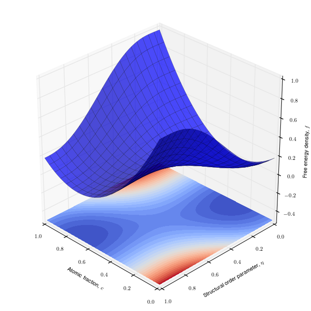
Parameter values
| Parameter | Value |
|---|---|
| 0.3 | |
| 0.7 | |
| 3 | |
| 3 | |
| 5 | |
| 1 | |
| 5 | |
| 5 | |
| 0.05 | |
| 0.5 | |
| 0.05 | |
| 0.1 | |
| 1.5 | |
| 0.1 |
Domain geometries and boundary conditions
Several boundary conditions, initial conditions and computational domain geometries are used to challenge different aspects of the numerical solver implementation. We test four combinations that are increasingly difficult to solve: two with square computational domains, see (a) and (b), with side lengths of 200 units, one with a computational domain in the shape of a “T,” see (c), with a total height of 120 units, a total width of 100 units, and horizontal and vertical section widths of 20 units, and one in which the computational domain is the surface of a sphere with a radius of r = 100 units, see (d). While most codes readily handle rectilinear domains, a spherical domain may pose problems, such as having the solution restricted to a two-dimensional curved surface. The coordinate systems and origins are given in Fig. 2. Periodic boundary conditions are applied to one square domain, see (a), while no-flux boundaries are applied to the other square domain, see (b), and the “T”-shaped domain, see (c). Periodic boundary conditions are commonly used with rectangular or rectangular prism domains to simulate an infinite material, while no-flux boundary conditions may be used to simulate an isolated piece of material or a mirror plane. As the computational domain is compact for the spherical surface, no boundary conditions are specified for it. Note that the same initial conditions are used for the square computational domains with no-flux, see (b), and periodic boundary conditions, see (a), such that when periodic boundary conditions are applied, there is a discontinuity in the initial condition at the domain boundaries.
(a) Square periodic
A 2D square domain with and periodic boundary conditions.
#PYTEST_VALIDATE_IGNORE_OUTPUT

from IPython.display import SVG

try:
    out = SVG(filename='../images/block1.svg')
except:
    out = None
out(b) Square no-flux
A 2D square domain with and no flux boundary conditions.
(c) T-shape
A T-shaped region with zero flux boundary conditions and with dimensions, and .
#PYTEST_VALIDATE_IGNORE_OUTPUT

from IPython.display import SVG

try:
    out = SVG(filename='../images/t-shape.svg')
except:
    out = None
out(d) Sphere
The domain is the surface of a sphere with radius 100.
Initial conditions
The initial conditions are chosen such that the average value of over the computational domain is approximately 0.5.
Initial conditions for (a), (b) and (c)
The initial value for on the square and “T” computational domains is specified by
where and . The intial value for on the square and “T” domain are given by,
where =0.1 and =1.5.
Figure 2: initial for (a), (b) and (c)
#PYTEST_VALIDATE_IGNORE_OUTPUT

import numpy as np
from bokeh.plotting import figure, show, output_file, output_notebook, gridplot
from bokeh.models import FixedTicker
output_notebook()
from bokeh.palettes import brewer, RdBu11, Inferno256
from bokeh.models.mappers import LinearColorMapper
import matplotlib as plt
import matplotlib.cm as cm
import numpy as np
from bokeh.models import HoverTool, BoxSelectTool

def generate_colorbar(mapper, width, height, n_ticks):
    high, low = mapper.high, mapper.low
    pcb = figure(width=width,
                 height=height,
                 x_range=[0, 1],
                 y_range=[low, high],
                 min_border_right=10)
    pcb.image(image=[np.linspace(low, high, 400).reshape(400,1)],
              x=[0],
              y=[low],
              dw=[1],
              dh=[high - low],
              color_mapper=mapper)
    pcb.xaxis.major_label_text_color = None
    pcb.xaxis.major_tick_line_color = None
    pcb.xaxis.minor_tick_line_color = None
    pcb.yaxis[0].ticker=FixedTicker(ticks=np.linspace(low, high, n_ticks))
    return pcb

def generate_contour_plot(data, xrange, yrange, width, height, mapper):
    p = figure(x_range=xrange, y_range=yrange, width=width, height=height, min_border_right=10)
    aa = p.image(image=[data],
                 x=xrange[0],
                 y=yrange[0],
                 dw=xrange[1] - xrange[0],
                 dh=yrange[1] - yrange[0],
                 color_mapper=mapper)
    return p


def get_data(xrange, yrange, data_func):
    N = 300
    xx, yy = np.meshgrid(np.linspace(xrange[0], xrange[1], N),
                         np.linspace(yrange[0], yrange[1], N))
    data = data_func(xx, yy)
    return xx, yy, data

def get_color_mapper(mpl_cm, high, low):
    colormap =cm.get_cmap(mpl_cm)
    bokehpalette = [plt.colors.rgb2hex(m) for m in colormap(np.arange(colormap.N))]
    mapper = LinearColorMapper(high=high,
                               low=low,
                               palette=bokehpalette)
    return mapper

def get_data_square(data_func):
    return get_data((0, 200), (0, 200), data_func)

def get_data_tshape(data_func):
    xx, yy, data = get_data((-40, 60), (0, 120), data_func)
    mask = ((xx < 0) | (xx > 20)) & (yy < 100)
    data[mask] = 0.5
    return xx, yy, data

def get_plot_grid(data_xy_func, high, low, n_ticks):
    mapper = get_color_mapper(cm.coolwarm, high, low)
    width, height = 300, 300

    all_plots = []
    for data_func in get_data_square, get_data_tshape:
        xx, yy, data = data_func(data_xy_func)
        contour_plot = generate_contour_plot(data,
                                             (xx.min(), xx.max()),
                                             (yy.min(), yy.max()),
                                             width,
                                             height,
                                             mapper)
        all_plots.append(contour_plot)

    all_plots.append(generate_colorbar(mapper, width // 4, height, n_ticks))
    return gridplot([all_plots])

def initial_concentration(x, y, epsilon=0.05, c_0=0.5):
    return c_0 + epsilon * (np.cos(0.105 * x) * np.cos(0.11 * y) + (np.cos(0.13 * x) * np.cos(0.087 * y))**2 \
                            + np.cos(0.025 * x - 0.15 * y) * np.cos(0.07 * x - 0.02 * y))

show(get_plot_grid(initial_concentration, 0.65, 0.35, 7),
     notebook_handle=True,
browser=None);Figure 3: initial for (a), (b) and (c)
#PYTEST_VALIDATE_IGNORE_OUTPUT

def initial_eta(x, y, epsilon_eta=0.1, psi=1.5, i=1):
    eta = epsilon_eta * (np.cos(0.01 * i * x - 4) * np.cos((0.007 + 0.01 * i) * y) \
                         + np.cos((0.11 + 0.01 * i) * x) * np.cos((0.11 + 0.01 * i) * y) \
                         + psi * (np.cos((0.046 + 0.001 * i) * x + (0.0405 + 0.001 * i) * y) \
                                  * np.cos((0.031 + 0.001 * i) * x - (0.004 + 0.001 * i) * y))**2)**2
    return eta

show(get_plot_grid(initial_eta, 1, 0, 6),
     notebook_handle=True,
browser=None);Initial conditions for (d)
The initial value of for the spherical computational domain is specified by
where and , and and are the polar and azimuthal angles, respectively, in a spherical coordinate system. These angles are translated into a Cartesian system as and dependent upon angle.
The intial value for for the spherical domain is specified by
where and enumerates the order parameters corresponding to the different phase variants.
Figure 4: initial for (d)
from mpl_toolkits.mplot3d import Axes3D
import numpy as np
from skimage import measure
import matplotlib.pyplot as plt
from matplotlib.tri import Triangulation
from matplotlib import ticker
import matplotlib.cm as cm


def get_geometry(R=100., NN=60):
    X, Y, Z = np.mgrid[-R * 1.1:R * 1.1:NN * 1j, -R * 1.1:R * 1.1:NN * 1j, -R * 1.1:R * 1.1:NN * 1j]
    surf_eq = np.sqrt(X**2 + Y**2 + Z**2) - R
    coords, triangles = measure.marching_cubes(surf_eq, 0)
    rescale = lambda xx: (2 * R * 1.1 * (np.array(xx) / (NN - 1) - 0.5)).ravel()
    return tuple(rescale(xx) for xx in zip(*coords)) + (triangles,)

def triangle_data(data_func, geometry):
    x, y, z, triangles = geometry
    return data_func(x, y, z)[triangles].mean(1)

def get_mpl_triangulation(geometry):
    x, y, z, triangles = geometry
    return Triangulation(x, y, triangles)

def make_colorbar(fig, collec):
    colorbar = fig.colorbar(collec, shrink=0.3)
    colorbar.locator = ticker.MaxNLocator(nbins=5)
    colorbar.update_ticks()

def plot_3d_sphere(data_func):
    geometry = get_geometry()
    fig = plt.figure(figsize=(8, 8))
    ax = fig.gca(projection='3d')
    collec = ax.plot_trisurf(get_mpl_triangulation(geometry),
                             geometry[2],
                             cmap=cm.coolwarm,
                             linewidth=0.0,
                             edgecolor="none")
    collec.set_array(triangle_data(data_func, geometry))
    collec.autoscale()
    ax.set_aspect('equal')
    ax.set_axis_off()
    make_colorbar(fig, collec)
    plt.show()

def conc_func(x, y, z, c_0=0.5, epsilon_sphere=0.05):
    r = np.sqrt(x**2 + y**2 + z**2)
    theta = np.arccos(z / r)
    phi = np.arctan(y / x)
    return c_0 + epsilon_sphere * (np.cos(8 * theta) * np.cos(15 * phi) \
                                   + (np.cos(12 * theta) * np.cos(10 * phi))**2 \
                                   + np.cos(2.5 * theta - 1.5 * phi) * np.cos(7 * theta - 2 * phi))

plot_3d_sphere(conc_func)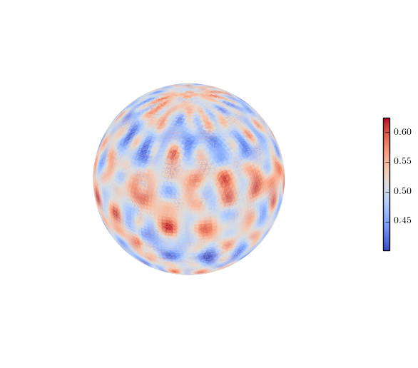
Figure 5: initial for (d)
def eta_func(x, y, z, epsilon_eta_sphere=0.1, psi=1.5, index=1):
    r = np.sqrt(x**2 + y**2 + z**2)
    theta = np.arccos(z / r)
    phi = np.arctan(y / x)
    return epsilon_eta_sphere * (
               np.cos(index * theta - 4) * np.cos((0.7 + index) * phi) \
               + np.cos((11 + index) * theta) * np.cos((11 + index) * phi) \
               + psi * (np.cos((4.6 + 0.1 * index) * theta + (4.05 + 0.1 * index) * phi) \
                        * np.cos((3.1 + 0.1 * index) * theta - (0.4 + 0.1 * index) * phi))**2)**2

plot_3d_sphere(eta_func)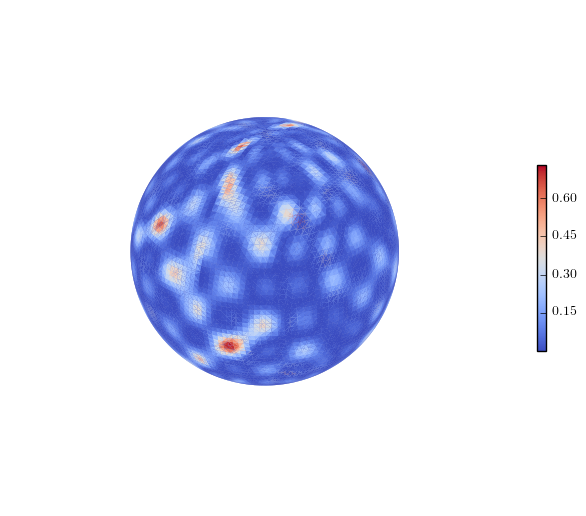
Results
Results from this benchmark problem are displayed on the [simulation result page]({{ site.baseurl }}/simulations) for different codes.
Feedback
Feedback on this benchmark problem is appreciated. If you have questions, comments, or seek clarification, please contact the [CHiMaD phase field community]({{ site.baseurl/community/ }}) through the [Gitter chat channel]({{ site.links.chat }}) or by [email]({{ site.baseurl }}/mailing_list/). If you found an error, please file an [issue on GitHub]({{ site.links.github }}/issues/new).
- Jokisaari, A. M., Voorhees, P. W., Guyer, J. E., Warren, J., & Heinonen, O. G. (2017). Benchmark problems for numerical implementations of phase field models. Computational Materials Science, 126, 139–151. 10.1016/j.commatsci.2016.09.022
- Zhu, J. Z., Wang, T., Ardell, A. J., Zhou, S. H., Liu, Z. K., & Chen, L. Q. (2004). Three-dimensional phase-field simulations of coarsening kinetics of γ′ particles in binary Ni–Al alloys. Acta Materialia, 52(9), 2837–2845. 10.1016/j.actamat.2004.02.032
- Wheeler, A. A., Boettinger, W. J., & McFadden, G. B. (1993). Phase-field model of solute trapping during solidification. Physical Review E, 47(3), 1893–1909. 10.1103/physreve.47.1893
- Kim, S. G., Kim, W. T., & Suzuki, T. (1999). Phase-field model for binary alloys. Physical Review E, 60(6), 7186–7197. 10.1103/physreve.60.7186
- Wheeler, A. A., Boettinger, W. J., & McFadden, G. B. (1992). Phase-field model for isothermal phase transitions in binary alloys. Physical Review A, 45(10), 7424–7439. 10.1103/physreva.45.7424
- Wheeler, A. A., Boettinger, W. J., & McFadden, G. B. (1992). Phase-field model for isothermal phase transitions in binary alloys. Physical Review A, 45(10), 7424–7439. 10.1103/physreva.45.7424
- Cahn, J. W. (1961). On spinodal decomposition. Acta Metallurgica, 9(9), 795–801. 10.1016/0001-6160(61)90182-1
- Elliott, C. M., French, D. A., & Milner, F. A. (1989). A second order splitting method for the Cahn-Hilliard equation. Numerische Mathematik, 54(5), 575–590. 10.1007/bf01396363
- Allen, S. M., & Cahn, J. W. (1979). A microscopic theory for antiphase boundary motion and its application to antiphase domain coarsening. Acta Metallurgica, 27(6), 1085–1095. 10.1016/0001-6160(79)90196-2