# from warnings import filterwarnings
# filterwarnings("ignore", category=UserWarning)
# filterwarnings("ignore", category=DeprecationWarning)

from IPython.display import HTML

HTML('''<script>
code_show=true;
function code_toggle() {
 if (code_show){
 $('div.input').hide();
 $('div.prompt').hide();
 } else {
 $('div.input').show();
$('div.prompt').show();
 }
 code_show = !code_show
}
$( document ).ready(code_toggle);
</script>
<form action="javascript:code_toggle()"><input type="submit" value="Code Toggle"></form>''')from IPython.display import HTML
HTML('''
<a href="{{ site.links.github }}/raw/nist-pages/benchmarks/benchmark1.ipynb"
download>
<button type="submit">Download Notebook</button>
</a>
''')Benchmark Problem 1: Spinodal Decomposition¶
from IPython.display import HTML

HTML('''{% include jupyter_benchmark_table.html num="[1]" revision=1 %}''')See the journal publication entitled “Benchmark problems for numerical implementations of phase field models” for more details about the benchmark problems. Furthermore, read the extended essay for a discussion about the need for benchmark problems.
Overview¶
Spinodal decomposition is one of the oldest problems in the phase field canon, and its formulation in terms of continuum fields goes back to the seminal works by Cahn and Hilliard [1]. The Cahn-Hilliard equation thus predates the name “phase field” in this context, but the term has subsequently been adopted by the community. While spinodal decomposition may be one of the simplest problems to model, it is highly relevant, as a large number of phase field models include the diffusion of a solute within a matrix. Furthermore, precipitation and growth may also be modeled with the same formulation if the appropriate initial conditions are chosen. For the benchmark problem, we select a simple formulation that is numerically tractable so that results may be obtained quickly and interpreted easily, testing the essential physics while minimizing model complexity and the chance to introduce coding errors.
Free energy and dynamics¶
The spinodal decomposition benchmark problem has a single order parameter, , which describes the atomic fraction of solute. The free energy of the system, , is expressed as
where is the chemical free energy density and is the gradient energy coefficient. For this problem, we choose to have a simple polynomial form,
such that is a symmetric double-well with minima at and , and controls the height of the double-well barrier. Because is symmetric (Fig. 1), and correspond exactly with the equilibrium atomic fractions of the and phases.
Figure 1: free energy density¶
%matplotlib inline
import matplotlib.pyplot as plt
import numpy as np

c_alpha = 0.3
c_beta = 0.7
rho_s = 5.

c = np.linspace(0, 1, 1000)
plt.figure(figsize=(6, 5))
plt.plot(c, rho_s * (c - c_alpha)**2 * (c - c_beta)**2, lw=4, color='k')
plt.xlabel("Atomic fraction, $c$", fontsize=20)
plt.ylabel("Free energy density, $f$", fontsize=20)
plt.xticks([0, 0.5, 1.0], fontsize=15)
plt.yticks([0, 0.1, 0.2], fontsize=15)
plt.show()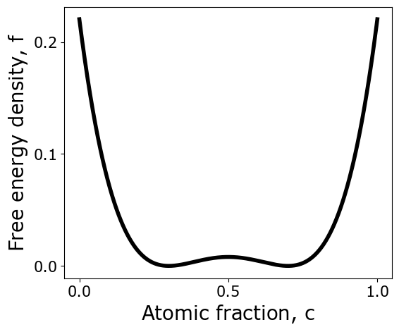
Because must obey a continuity equation -- the flux of is conserved -- the evolution of is given by the Cahn-Hilliard equation [1], which is derived from an Onsager force-flux relationship [ 2 ]:
where is the mobility of the solute. For simplicity, both the mobility and the interfacial energy are isotropic. We choose , , , , and . Because the interfacial energy, diffuse interface width, and free energy parameterization are coupled, we obtain the diffuse interface width of units over which varies as , and an interfacial energy [3].
Parameter values¶
| Parameter | Value |
|---|---|
| 0.3 | |
| 0.7 | |
| 5 | |
| 2 | |
| 5 | |
| 0.01 | |
| 0.05 | |
| 0.5 |
Domain geometries and boundary conditions¶
Several boundary conditions, initial conditions and computational domain geometries are used to challenge different aspects of the numerical solver implementation. We test four combinations that are increasingly difficult to solve: two with square computational domains, see (a) and (b), with side lengths of 200 units, one with a computational domain in the shape of a “T,” see (c), with a total height of 120 units, a total width of 100 units, and horizontal and vertical section widths of 20 units, and one in which the computational domain is the surface of a sphere with a radius of r = 100 units, see (d). While most codes readily handle rectilinear domains, a spherical domain may pose problems, such as having the solution restricted to a two-dimensional curved surface. The coordinate systems and origins are given in Fig. 2. Periodic boundary conditions are applied to one square domain, see (a), while no-flux boundaries are applied to the other square domain, see (b), and the “T”-shaped domain, see (c). Periodic boundary conditions are commonly used with rectangular or rectangular prism domains to simulate an infinite material, while no-flux boundary conditions may be used to simulate an isolated piece of material or a mirror plane. As the computational domain is compact for the spherical surface, no boundary conditions are specified for it. Note that the same initial conditions are used for the square computational domains with no-flux, see (b), and periodic boundary conditions, see (a), such that when periodic boundary conditions are applied, there is a discontinuity in the initial condition at the domain boundaries.
(a) Square periodic¶
A 2D square domain with and periodic boundary conditions.
#PYTEST_VALIDATE_IGNORE_OUTPUT

from IPython.display import SVG
try:
    out = SVG(filename='../images/block1.svg')
except:
    out = None
out(b) Square no-flux¶
A 2D square domain with and no flux boundary conditions.
(c) T-shape¶
A T-shaped region with zero flux boundary conditions and with dimensions, and .
#PYTEST_VALIDATE_IGNORE_OUTPUT

from IPython.display import SVG
try:
    out = SVG(filename='../images/t-shape.svg')
except:
    out = None
out(d) Sphere¶
The domain is the surface of a sphere with radius 100.
Initial conditions¶
The initial conditions for the first benchmark problem are chosen such that the average value of over the computational domain is approximately 0.5.
Initial conditions for (a), (b) and (c)¶
Figure 2: initial for (a), (b) and (c)¶
#PYTEST_VALIDATE_IGNORE_OUTPUT

import numpy as np
from bokeh.plotting import figure, show, output_file, output_notebook, gridplot
from bokeh.models import FixedTicker
output_notebook()
from bokeh.palettes import brewer, RdBu11, Inferno256
from bokeh.models.mappers import LinearColorMapper
import matplotlib as plt
import matplotlib.cm as cm
import numpy as np
from bokeh.models import HoverTool, BoxSelectTool

def generate_colorbar(mapper, width, height, n_ticks):
    high, low = mapper.high, mapper.low
    pcb = figure(width=width,
                 height=height,
                 x_range=[0, 1],
                 y_range=[low, high],
                 min_border_right=10)
    pcb.image(image=[np.linspace(low, high, 400).reshape(400,1)],
              x=[0],
              y=[low],
              dw=[1],
              dh=[high - low],
              color_mapper=mapper)
    pcb.xaxis.major_label_text_color = None
    pcb.xaxis.major_tick_line_color = None
    pcb.xaxis.minor_tick_line_color = None
    pcb.yaxis[0].ticker=FixedTicker(ticks=np.linspace(low, high, n_ticks))
    return pcb

def generate_contour_plot(data, xrange, yrange, width, height, mapper):
    p = figure(x_range=xrange, y_range=yrange, width=width, height=height, min_border_right=10)
    aa = p.image(image=[data],
                 x=xrange[0],
                 y=yrange[0],
                 dw=xrange[1] - xrange[0],
                 dh=yrange[1] - yrange[0],
                 color_mapper=mapper)
    return p


def get_data(xrange, yrange, data_func):
    N = 300
    xx, yy = np.meshgrid(np.linspace(xrange[0], xrange[1], N),
                         np.linspace(yrange[0], yrange[1], N))
    data = data_func(xx, yy)
    return xx, yy, data

def get_color_mapper(mpl_cm, high, low):
    colormap =cm.get_cmap(mpl_cm)
    bokehpalette = [plt.colors.rgb2hex(m) for m in colormap(np.arange(colormap.N))]
    mapper = LinearColorMapper(high=high,
                               low=low,
                               palette=bokehpalette)
    return mapper

def get_data_square(data_func):
    return get_data((0, 200), (0, 200), data_func)

def get_data_tshape(data_func):
    xx, yy, data = get_data((-40, 60), (0, 120), data_func)
    mask = ((xx < 0) | (xx > 20)) & (yy < 100)
    data[mask] = 0.5
    return xx, yy, data

def get_plot_grid(data_xy_func, high, low, n_ticks):
    mapper = get_color_mapper(cm.coolwarm, high, low)
    width, height = 300, 300

    all_plots = []
    for data_func in get_data_square, get_data_tshape:
        xx, yy, data = data_func(data_xy_func)
        contour_plot = generate_contour_plot(data,
                                             (xx.min(), xx.max()),
                                             (yy.min(), yy.max()),
                                             width,
                                             height,
                                             mapper)
        all_plots.append(contour_plot)

    all_plots.append(generate_colorbar(mapper, width // 4, height, n_ticks))
    return gridplot([all_plots])

def initial_concentration(x, y, epsilon=0.01, c_0=0.5):
    return c_0 + epsilon * (np.cos(0.105 * x) * np.cos(0.11 * y) + (np.cos(0.13 * x) * np.cos(0.087 * y))**2 \
                            + np.cos(0.025 * x - 0.15 * y) * np.cos(0.07 * x - 0.02 * y))

show(get_plot_grid(initial_concentration, 0.53, 0.47, 7),
     notebook_handle=True,
browser=None);Initial conditions for (d)¶
The initial value of for the spherical computational domain is specified by
where , and and are the polar and azimuthal angles, respectively, in a spherical coordinate system. These angles are translated into a Cartesian system as and dependent upon angle.
Figure 3: initial for (d)¶
from mpl_toolkits.mplot3d import Axes3D
import numpy as np
from skimage import measure
import matplotlib.pyplot as plt
from matplotlib.tri import Triangulation
from matplotlib import ticker
import matplotlib.cm as cm


def get_geometry(R=100., NN=60):
    X, Y, Z = np.mgrid[-R * 1.1:R * 1.1:NN * 1j, -R * 1.1:R * 1.1:NN * 1j, -R * 1.1:R * 1.1:NN * 1j]
    surf_eq = np.sqrt(X**2 + Y**2 + Z**2) - R
    coords, triangles, _, _ = measure.marching_cubes(surf_eq, 0)
    rescale = lambda xx: (2 * R * 1.1 * (np.array(xx) / (NN - 1) - 0.5)).ravel()
    return tuple(rescale(xx) for xx in zip(*coords)) + (triangles,)

def triangle_data(data_func, geometry):
    x, y, z, triangles = geometry
    return data_func(x, y, z)[triangles].mean(1)

def get_mpl_triangulation(geometry):
    x, y, z, triangles = geometry
    return Triangulation(x, y, triangles)

def make_colorbar(fig, collec):
    colorbar = fig.colorbar(collec, shrink=0.3)
    colorbar.locator = ticker.MaxNLocator(nbins=5)
    colorbar.update_ticks()

def plot_3d_sphere(data_func):
    geometry = get_geometry()
    fig = plt.figure(figsize=plt.figaspect(0.5) * 1.5)
    ax = fig.add_subplot(projection='3d')
    collec = ax.plot_trisurf(get_mpl_triangulation(geometry),
                             geometry[2],
                             cmap=cm.coolwarm,
                             linewidth=0.0,
                             edgecolor="none")
    collec.set_array(triangle_data(data_func, geometry))
    collec.autoscale()
    ax.set_aspect('auto')
    ax.set_axis_off()
    make_colorbar(fig, collec)
    plt.show()

def conc_func(x, y, z, c_0=0.5, epsilon_sphere=0.05):
    r = np.sqrt(x**2 + y**2 + z**2)
    theta = np.arccos(z / r)
    phi = np.arctan(y / x)
    return c_0 + epsilon_sphere * (np.cos(8 * theta) * np.cos(15 * phi) \
                                   + (np.cos(12 * theta) * np.cos(10 * phi))**2 \
                                   + np.cos(2.5 * theta - 1.5 * phi) * np.cos(7 * theta - 2 * phi))

plot_3d_sphere(conc_func)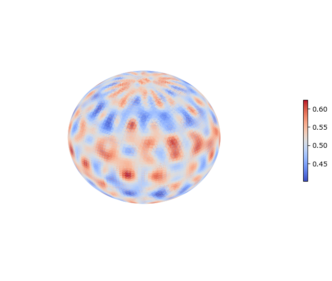
Submission Guidelines¶
Please follow these upload instructions.
In addition to that specified, further data to upload can include a YouTube video, snapshots of the simulation at different times, or the field variable at each point in the entire domain at different times. This auxiliary data is not required, but will help others view your work.
Part (a)¶
Part (a) requires running the simulation to equilibrium, and the following data should be collected.
The free energy integrated over the whole domain, , at each timestep.
The free energy data should be recorded in a file named
free_energy_1a.csv. This plain-text CSV file (comma-separated values) must have the following format -- note the column headings and lack of spaces:time,free_energy 0.00000000,319.0337102 5.00000000,318.8273928 ... 10000.0000,40.81065093 ...The composition field, , at each grid point in the domain at the following times (aspirational):
1,000
10,000
100,000
1,000,000
You may provide this data in whatever format you consider “most useful,” e.g. a checkpoint file in the format native to your phase-field simulation framework, and the PFHub operations team will attempt to handle it correctly. Optionally, please consider also uploading a VTK ImageData file. If your mesh is unstructured or irregular, this will require appropriate interpolation prior to export. This can be accomplished using common scientific visualization software, e.g. using the PointVolumeInterpolator filter in ParaView.‡
The names of these data files should encode the time and problem, e.g.,
raw_data_1a.0001000.vti,raw_data_1a.0010000.vti,raw_data_1a.0100000.vti, andraw_data_1a.1000000.vti.
‡: Any mention of commercial products within NIST web pages is for information only; it does not imply recommendation or endorsement by NIST.
Parts (b) through (d)¶
The same data as in Part (a) are required, stored in appropriately named files: please follow the same instructions, modifying “1a” with the appropriate letter (“1b”, “1c”, etc.).
Results¶
Results from this benchmark problem are displayed on the [simulation result page]({{ site.baseurl }}/simulations) for different codes.
Feedback¶
Feedback on this benchmark problem is appreciated. If you have questions, comments, or seek clarification, please contact the [CHiMaD phase field community]({{ site.baseurl }}/community/) through the [Gitter chat channel]({{ site.links.chat }}) or by [email]({{ site.baseurl }}/mailing_list/). If you found an error, please file an [issue on GitHub]({{ site.links.github }}/issues/new).
- Jokisaari, A. M., Voorhees, P. W., Guyer, J. E., Warren, J., & Heinonen, O. G. (2017). Benchmark problems for numerical implementations of phase field models. Computational Materials Science, 126, 139–151. 10.1016/j.commatsci.2016.09.022
- Cahn, J. W. (1961). On spinodal decomposition. Acta Metallurgica, 9(9), 795–801. 10.1016/0001-6160(61)90182-1
- Cahn, J. W. (1961). On spinodal decomposition. Acta Metallurgica, 9(9), 795–801. 10.1016/0001-6160(61)90182-1
- Balluffi, R. W., Allen, S. M., & Carter, W. C. (2005). Kinetics of Materials. Wiley. 10.1002/0471749311
- Cahn, J. W., & Hilliard, J. E. (1958). Free Energy of a Nonuniform System. I. Interfacial Free Energy. The Journal of Chemical Physics, 28(2), 258–267. 10.1063/1.1744102