Larry Aagesen (Larry Aagesen), David Montiel, Sourabh Kadambi (Sourabh Kadambi), Sudipta Biswas (Sudipta Biswas)
After the phase field model formulation is developed, implemented in code, and verified, it can be set up to solve the scientific/engineering problem of interest. The purpose of this page is to give guidance on some of the important considerations when setting up your code to solve your specific problem, organized in the following sections:
Spatial dimension (1D vs. 2D vs. 3D)
Spatial Dimension
In setting up a phase field simulation, it is important to understand the role of spatial dimensions in the physics governing the problem, and how that might impact the simulation results and its interpretation. This is particularly important if simulations are being performed in reduced dimensions compared to the actual dimension of the problem, which is a common practice employed to reduce the computational costs.
It is likely that the physical behavior of a certain phenomenon might scale differently in 1D, 2D and 3D. This could be related to the physical processes in the bulk regions of the system or at the interfacial regions, or both. For instance, the amount of interfacial region relative to the bulk phase region differs in 1D, 2D and 3D, and also governs many physical aspects of material behavior.
Therefore, it is important to determine how reduced dimensionality might affect predictions or comparison of simulation results with reality. In certain situations, on the other hand, it might be appropriate to setup the problem in reduced dimensions of 1D or 2D due to the inherent symmetry or directionality in the problem. Moreover, for simple microstructure geometries, it might be possible to setup the model in cylindrical or spherical coordinates, which can allow the simplicity of 1D computations while also capturing 2D and 3D behavior of the model accurately.
Example
To demonstrate a case where simulation outcomes can significantly differ in different dimensions, we consider the single seed case of the homogeneous nucleation benchmark problem. A simple phase field model with a single non-conserved order parameter describes an isothermal pure substance with one liquid phase (order parameter = 0) and one solid phase (order parameter = 1). The nucleation driving force for the solid phase is . The free energy of the diffuse interface is .
We consider a seed nucleus of 7.5 unit radius in 2D and 3D. The 2D simulation domain is of size , and the 3D simulation domain is of size . The nucleus is centered at . Uniform mesh of element size is used. Neumann boundary conditions, given by the zero normal-derivative of the order parameter, are applied on all domain boundaries. Figure 1 and Figure 2 below show the starting geometry of the nucleus in 2D and 3D.
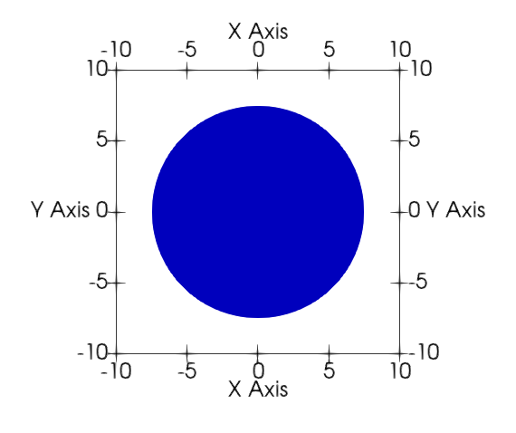
Figure 1:The 2D representation of the 2D case of the homogeneous nucleation problem.
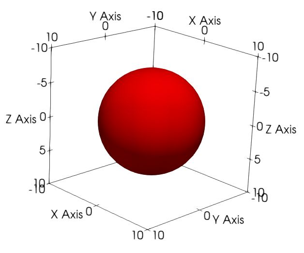
Figure 2:The 3D representation of the 2D case of the homogeneous nucleation problem.
The time evolution of the order parameter, given by the Allen-Cahn equation, was solved using the MOOSE framework. Details of the numerical method can be found in Wu et al. (2021). The simulations results of nucleus evolution are shown in the figures below: (left) order parameter profile measured radially from the center of domain at different evolution times; (right) radius as a function of evolution time. In Figure 3 and Figure 4, we see that the seed of same starting radius units evolves starkly differently in 2D and 3D. While the nucleus grows in 2D, it shrinks and dissolves in 3D.
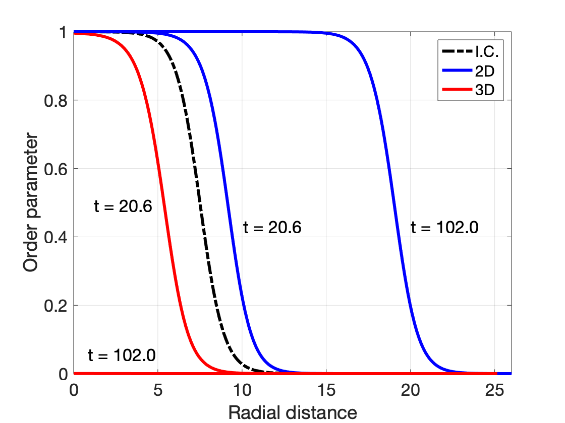
Figure 3:Order Parameter v. Radial Distance
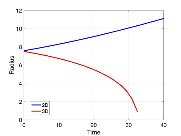
Figure 4:Radius v. Time
The role of dimensionality in homogeneous nucleation can be understood from the classical nucleation theory where the solid-liquid interface is modeled as a mathematically sharp interface. The interface is a 1D line in a 2D system and a 2D plane in a 3D system. The free energy of the nucleus particle is a balance between the energy cost in forming the interface, and the energy released due to the driving force in forming the bulk particle. For a 2D system, . For a 3D system, . When the rate of change of free energy with respect to particle size is negative, the particle is favored to grow; otherwise it will shrink and dissolve. By setting , we obtain the critical radius as in 2D and in 3D.
We can now apply the above sharp-interface analysis to our diffuse interface approximation in the phase field model. For the given model parameters, we obtain units in 2D and units in 3D. In our simulation setup of units, in 2D, but in 3D. Therefore, the nucleus is favored to grow in 2D but shrinks in 3D as observed in the simulations, see Figure 5 and Figure 6.
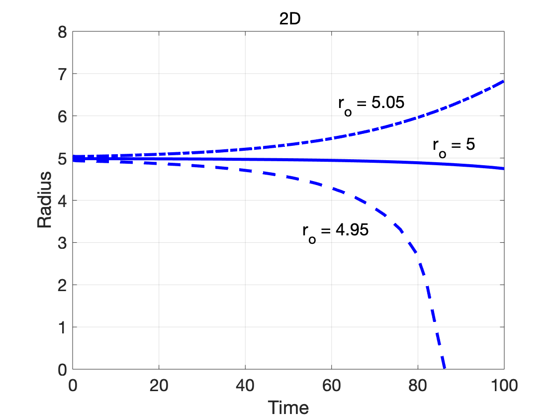
Figure 5:2D Radius v. Time
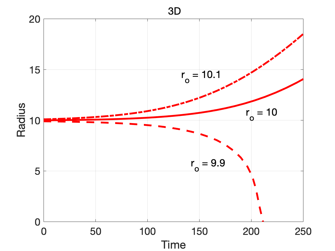
Figure 6:3D Radius v. Time
The dependence on dimensionality is further illustrated by considering cases where the initial radius is close to the critical radius: , and . The simulation results of radius evolution are in Figs. Figure 5 and Figure 6 for 2D and 3D, respectively. As expected from the the classical homogeneous nucleation theory, the sub-critical nucleus with shrinks and the super-critical nucleus with grows.
Since the nucleus in the phase field model is a diffuse-interface approximation of the classical sharp interface nucleus, is fairly close to an unstable equilibrium. Ideally, the radius would remain constant with time. However, since the system is unstable, small numerical errors accumulate with time, eventually leading to growth or shrinkage of the nucleus. During initial time steps, the interface profile is expected to undergo some changes from the starting profile due to equilibration. While the function is a common choice for the initial condition of the interface, it is an exact solution only for a planar interface, representative of a 1D scenario.
Initial conditions
For simulations of the evolution of two or more phases, it is important to anticipate the expected equilibrium state of the system given the initial conditions. To do this, one needs the phase diagram as determined by the bulk contribution of the free energy density.
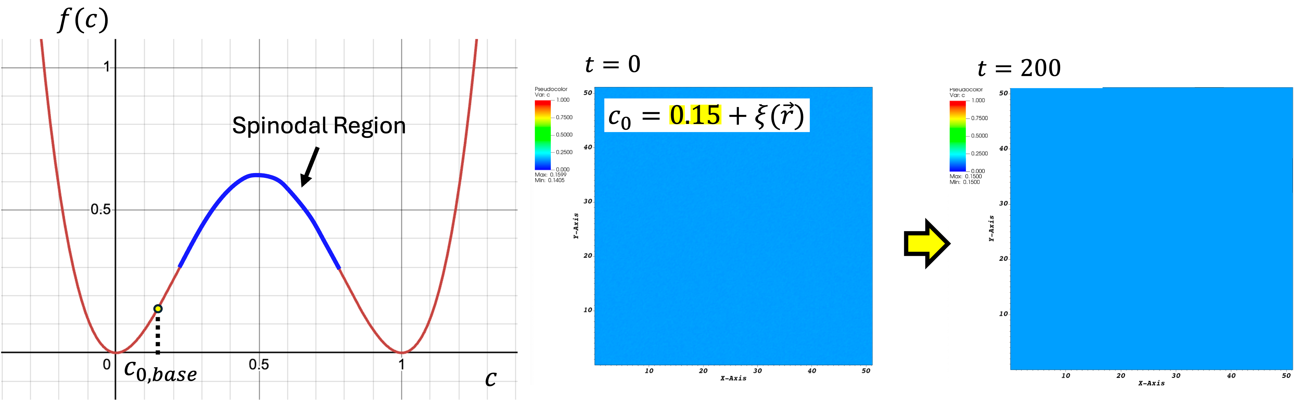
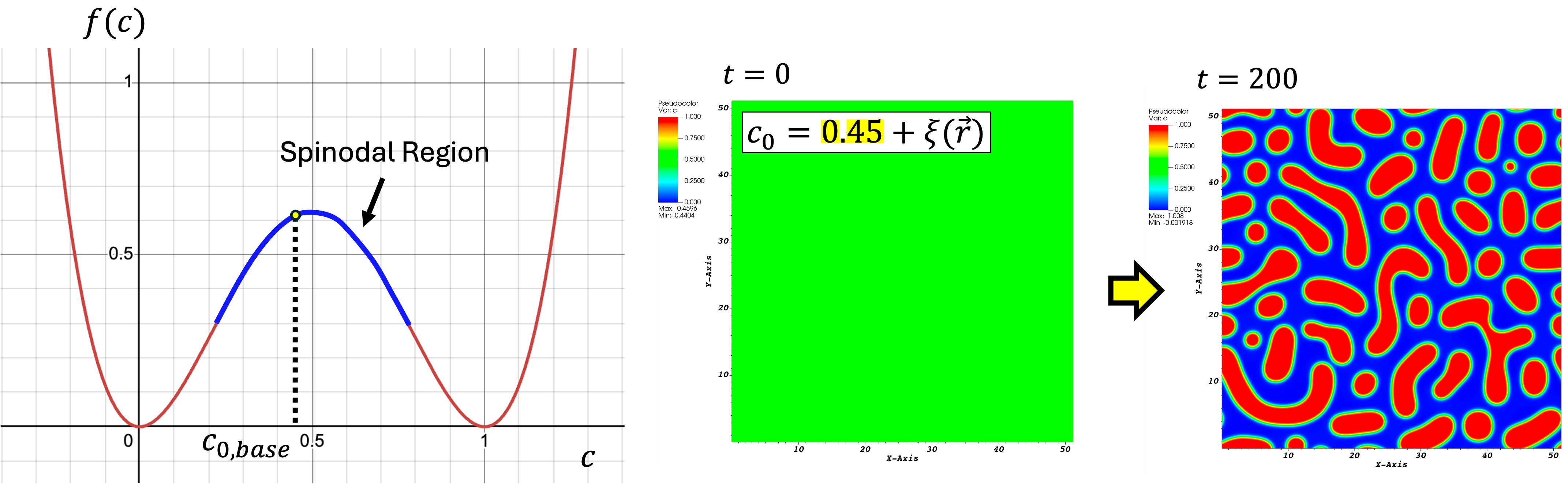
For example, in simulating phase separation following spinodal decomposition, it is common to define the initial state of the order parameter as a spatially uniform field with an added small ‘noisy’ perturbation with small amplitude. However, this order parameter must be within the spinodal region of the phase diagram, i.e., the region where spontaneous decomposition leads to a decrease in the free energy. Below we show two instances that demonstrate that choosing different values for the baseline order parameter, , and the same initial perturbation term, , for the initial conditions of leads to different dynamics.
Boundary conditions
Boundary conditions (BC) are required to solve for the governing equations in all phase field simulations. In general, every field must have a defined BC at every boundary of the system. The three most common types of boundary conditions for phase field simulation are:
Dirichlet BC: The value of a field is specified at the boundary. This type of boundary condition is useful whenever we want to impose a value to an order parameter or field at one or more boundaries. Some common examples include setting a constant value for temperature to simulate a heat reservoir, or setting a constant value for a solid/liquid order parameter to indicate a fixed phase beyond the confines of the system.
Neumann BC: The value of the spatial derivative of a field is specified at the boundary. This type of boundary condition is useful to specify fluxes of fields at the boundary. For example, setting the natural BC (a special case of Neumann BC) for a field at the boundary enforces the normal component of gradient of that field to be zero along that boundary. Therefore, if a flux for that field is proportional to this gradient, natural BC is equivalent to imposing zero flux at the boundary. This BC is convenient to ensure that the field is conserved. In addition, natural BCs are useful to exploit known symmetries in the morphology of domains. For example, a spherical domain can be simulated using a quarter (in 2D) or eighth of a system (in 3D) by placing centering the sphere in a corner of the system and imposing natural BCs along the boundaries that define the corner.
Periodic BCs: The value of the field in a boundary with a periodic BC matches the value from the opposite boundary. These types of BCs are useful to simulate periodic domains, but also to minimize boundary effects since the system does not interact with borders.
Try different boundary conditions and check their impact
We used the results from Benchmark Problem 1a and Problem 1b to analyze the effect of boundary conditions. In addition, we solved for Cahn-Hilliard dynamics under the same initial condition and simulation parameters as problem 1 but using mixed boundary conditions, i.e., different boundary conditions for each boundary. We compare the results for each case at simulation time t = 1000. The simulations were carried out in the PRISMS-PF framework using a uniform square mesh with linear elements and a time step, = 0.005. The results are shown in Figure 7.
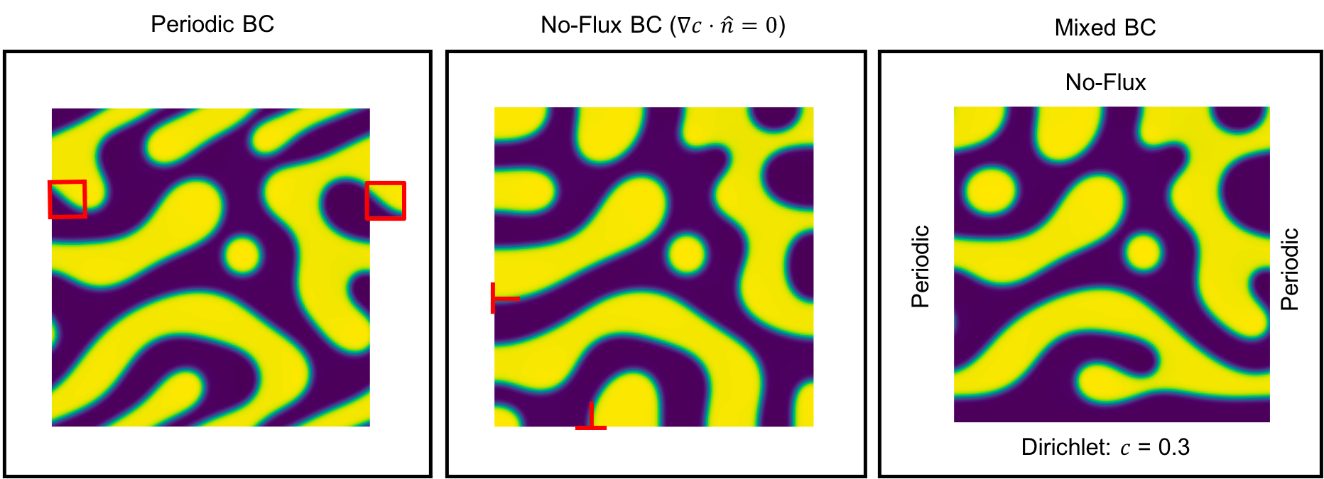
Figure 7:Comparison of results for benchmark 1
As can be seen in Figure 7, for periodic boundaries the - domains are continuous on opposite sides of the system. For no-flux boundaries, the - interfaces are normal to the boundary. For Dirichlet boundaries (bottom boundary of the right panel), the value of c is fixed along the boundary.
Interface width
Phase field modeling is a diffuse interface approach, meaning that interfaces are represented by a smooth variation of one or more order parameters across the interface. The width of the interface is a function of the model parameters and the interface width is determined by model parameter choices. In some cases, an analytical expression is available that relates interface width to phase field model parameters (such as free energy barrier height and gradient energy coefficient, which also impact the interfacial energy). In other cases, no analytical solution is available and the interface width must be approximated or determined numerically based on parameter choices. Such details are specific to the formulation being used.
Once the relationship between model parameters and interface width is understood, an appropriate selection of interface width needs to be made (while maintaining the correct interfacial energy for the system being studied). In some cases, the interface width in the phase field model can be chosen to match the actual physical width of the interface being studied (typically sub-nanometer). However, resolving a physically realistic interface width requires a sub-nanometer grid/mesh (grid/mesh convergence is described further in the next section). Using a physically realistic interface width often makes it computationally unfeasible to simulate systems large enough to be statistically representative. Therefore, in many cases an interfacial width that is much larger than the the physical width of an interface is used. In these cases, a careful balance between computational efficiency and model accuracy is needed; the interface width should be chosen to be small enough that the physics of the system are accurately represented, while maintaining adequate computational performance. A useful rule of thumb as a starting point is that the interface width should be at least an order of magnitude smaller than the smallest microstructural feature size of interest. Starting from this guideline, simulations of microstructural evolution with varying interface widths can be run to ensure that the choice of interface width does not affect the simulation results. A small test problem may be useful for testing convergence with respect to interface width; for example a shrinking circular grain embedded in another grain may be used for testing convergence of a grain growth model with respect to interface width rather than starting with large, costly simulations with hundreds of grains.
Convergence studies
Carry out grid/mesh convergence study AFTER you have finalized your interfacial width.
As an example of a mesh convergence study, we can consider Benchmark Problem 1 from the Phase Field Community Hub. In this problem, which models spinodal decomposition using the Cahn-Hilliard equation, the width of the diffuse interface is 4.47, as defined by the Cahn-Hilliard equation and physical parameters in the problem statement. Given this interface width, we need to ensure there are a sufficient number of grid points (for finite difference schemes) or mesh elements (for finite element or finite volume schemes) through the diffuse interface to adequately resolve the variation of the composition order parameter.
In Problem 1b, a square domain with dimensions and no-flux boundary conditions is considered. An example of a mesh convergence study for this problem using the MOOSE framework phase field module (a finite element code) is described. The domain is discretized using increasing numbers of elements in the direction and in the direction, maintaining for square elements (using linear Lagrange shape functions). The simulations with varying numbers of elements are run until a significant amount of microstructural evolution has occurred. We need to increase the number of elements until the microstructure at a fixed time no longer changes with further increases in the number of elements; at this point the simulation is converged with respect to the mesh resolution.
The simulation initial conditions and the microstructures at are shown in Figure 8.
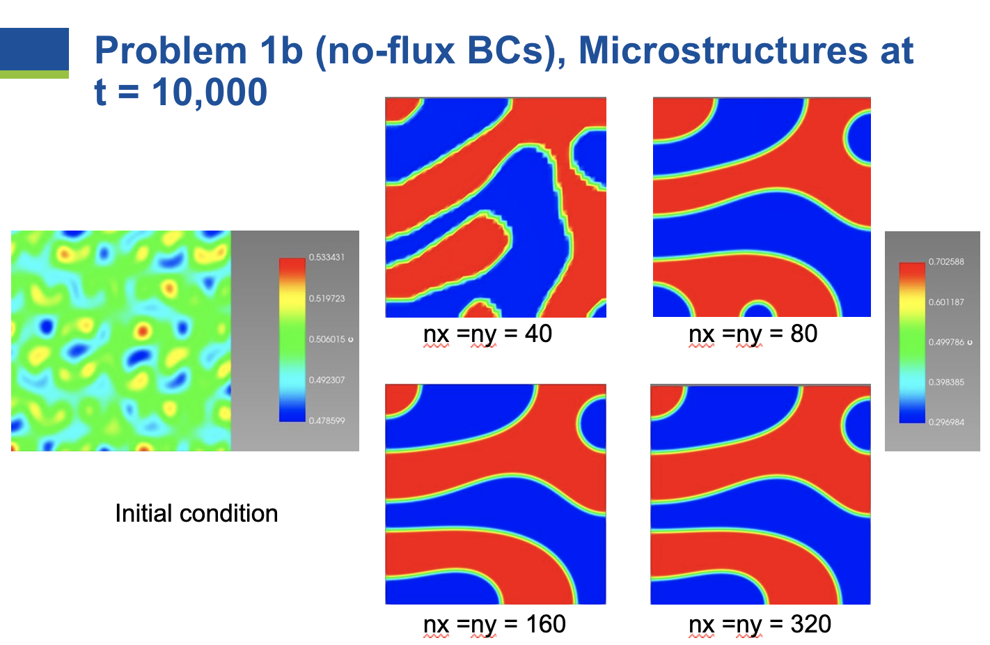
Figure 8:Problem 1b (no-flux BCs).
As the number of elements in each direction is increased from 40 to 80 to 160, changes in the microstructure are observed. However, once the number of elements increases to 320, no further changes are observed in the microstructure. Therefore, the problem is converged with respect to mesh resolution at . For this number of elements, each element has size = 200 / 160 = 1.25. Therefore, the number of elements through the diffuse interface width is 4.47 / 1.25 = 3.6. Practical experience in the phase field community has shown that somewhere between 3 to 5 elements through the interface are usually required to obtain mesh convergence; however, the appropriate resolution is problem-specific, and convergence should be tested for the specific physics and parameters at hand.
Carry out time step convergence studies. Try higher-order schemes, adaptive time stepping, etc. For explicit time integration, know your stability limit.
For codes that use explicit time integration, there is a maximum value of the time step beyond which the solution becomes numerically unstable. This stability limit can be determined by the Courant–Friedrichs–Lewy (CFL) condition and, in general, it strongly depends on the order of the spatial derivatives. Figure 9 shows the simulation results for Benchmark Problem 1b using time step values slightly below and slightly above the stability limit. We employed a forward Euler time-integration scheme and spatially discretized the system using first order elements. The simulations were performed in the PRISMS-PF framework. The left panel of the figure below shows a snapshot of the concentration at time , which was obtained using a stable time step of . If the time step is increased to , the time step goes above the stability limit. The right panel shows the concentration at time for and features a numerical instability that appears near the bottom boundary. After only four time steps the amplification of this instability caused the simulation to fail.
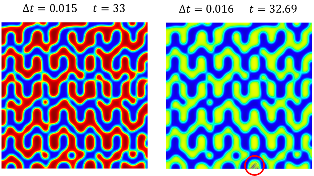
Figure 9:Simulation results for Benchmark Problem 1b
Codes that use implicit time stepping schemes may have fewer restrictions with respect to stability as time step size is increased, depending on the problem. However, discretization error still occurs in implicit schemes and increases with the size of the time step taken. Therefore, a convergence study should be carried out to ensure that the size of the time step does not affect the simulation results. As an example, we can again consider Benchmark Problem 1 from the Phase Field Community Hub. Problem 1b was solved with the phase field module from the MOOSE framework using . Figure 10 shows the results. The microstructure at remains the same for , , and . Some differences in the microstructure are observed at , and further differences become apparent at . In practice, it is recommended to start with a given time step and gradually decrease it until no changes are apparent with further decreases in time step size.
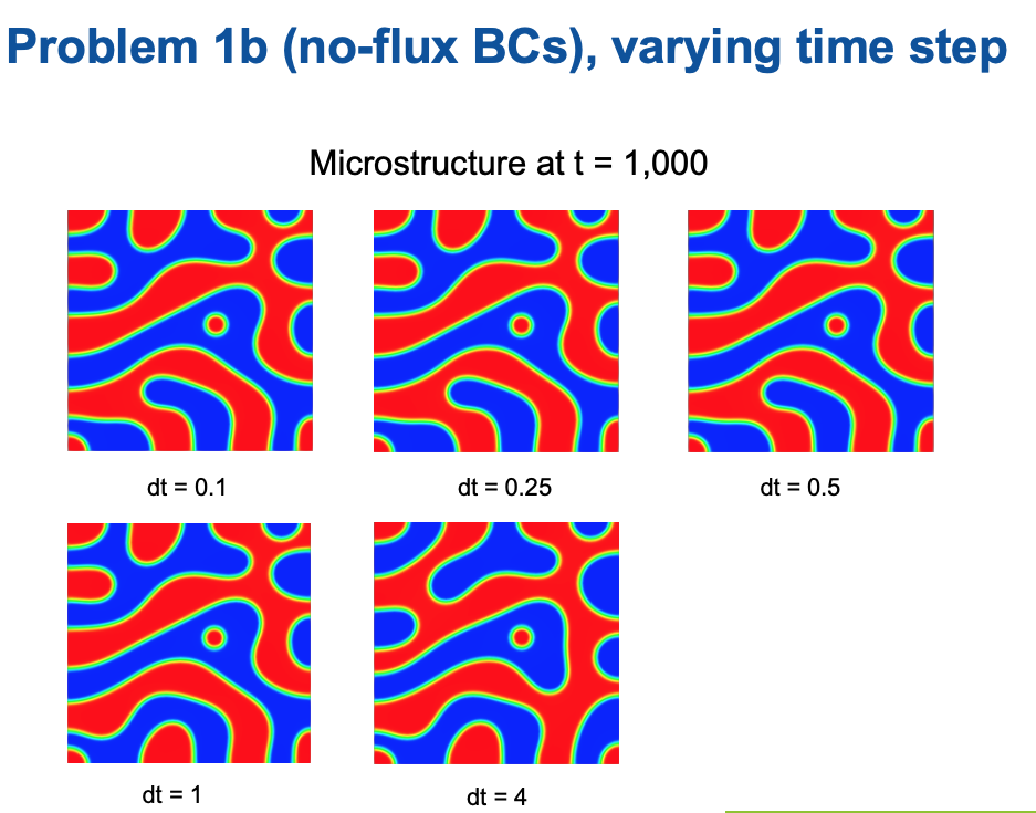
Figure 10:Problem 1b (no-flux BCs), varying time step
Adaptive time stepping can be useful to increase the time step size
during time periods in the simulation where there are fewer
microstructural changes, particularly for codes that use implicit time
stepping schemes. However, convergence must still be checked for the
parameters of the time stepping scheme being used. An example is the
IterationAdaptiveDt time stepping scheme used in the MOOSE
framework. This scheme attempts to increase or decrease the time step
to keep the solver using a certain number of nonlinear iterations
(controlled by the parameter optimal_iterations), within a window or
plus or minus the parameter iteration_window. Higher values of
optimal_iterations parameter result in higher time steps, and with
that comes the risk of discretization error changing simulation
results. Figure 11 shows the results for Problem 1b,
optimal_iterations values of 6 or 8 gave results consistent with the
converged time step of 0.5, but when optimal_iterations was
significantly increased to 15, changes in the microstructure resulted.
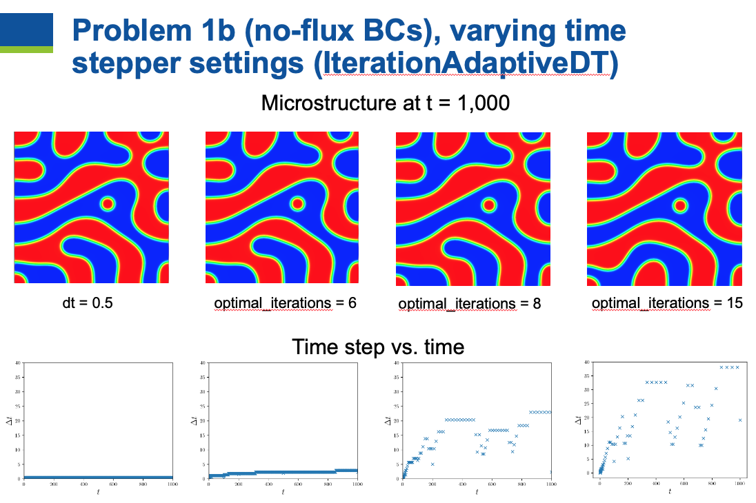
Figure 11:Problem 1b (no-flux BCs), adaptive time-stepping
Impact of Orientation
Oftentimes, the results of the phase field simulations are sensitive to the orientation and alignment of the key microstructural features with the mesh/grid points. To demonstrate this we pick a simple solidification problem with dendritic structure formation. In this case, we utilize the solidification example from the MOOSE-based phase field module. This example problem can quickly demonstrate dendritic structure formation including the formation of secondary dendritic arms in a computationally cost-effective manner. Here, we use 4-fold symmetry of the structure and vary the reference angles to misorient the dendritic arms with respect to the mesh. Figure 12 and Figure 13 show structures corresponding to and reference angle is presented below:
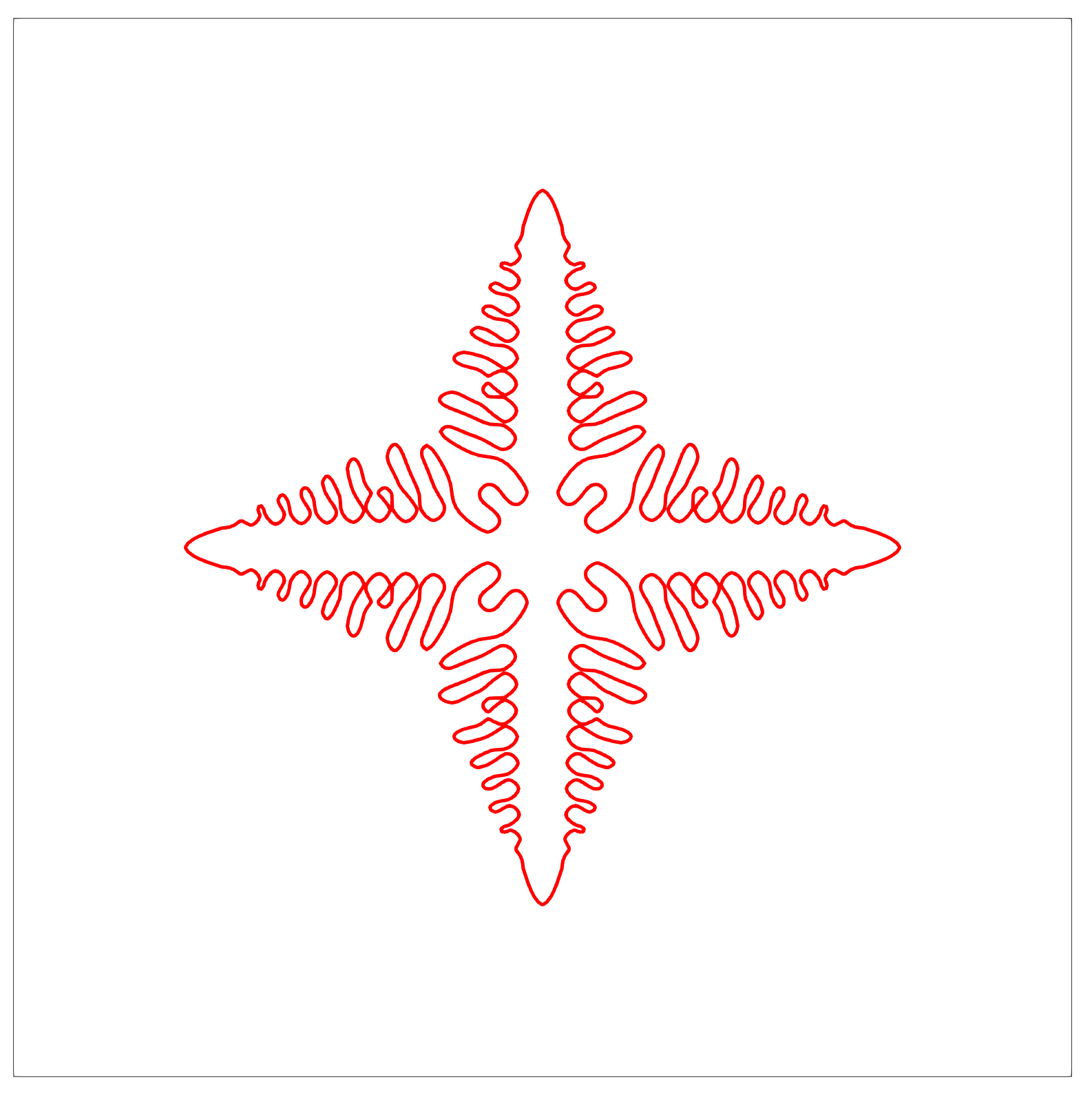
Figure 12:Dendritic structure oriented with the grid.
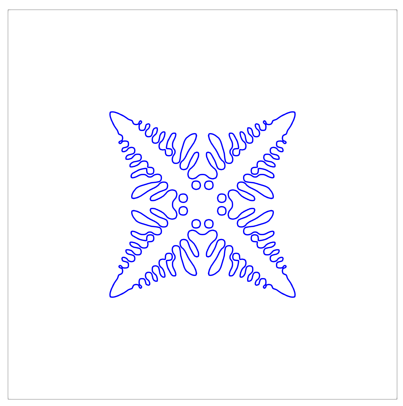
Figure 13:Dendritic structure oriented at to the grid.
It is noteworthy that the shape of the dendrite varies with orientation (as observed by the difference in the dendrite center). For better comparison, we rotate the dendrite to align the primary dendrite arms with the reference orientation dendrite (see Figure 14):
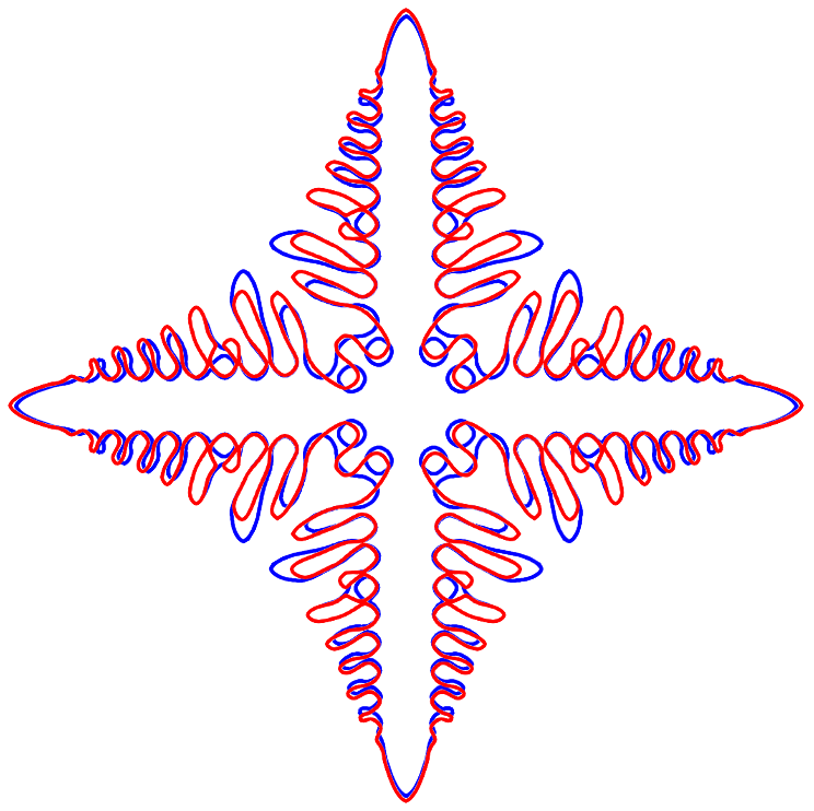
Figure 14:Dendritic structure superimposed.
This highlights the slight differences between the dendrite shapes, especially the center and the secondary dendritic arms. Additionally, the growth rate of the solid also varies with orientation as observed by the change in solid area fraction over time (see Figure 15):
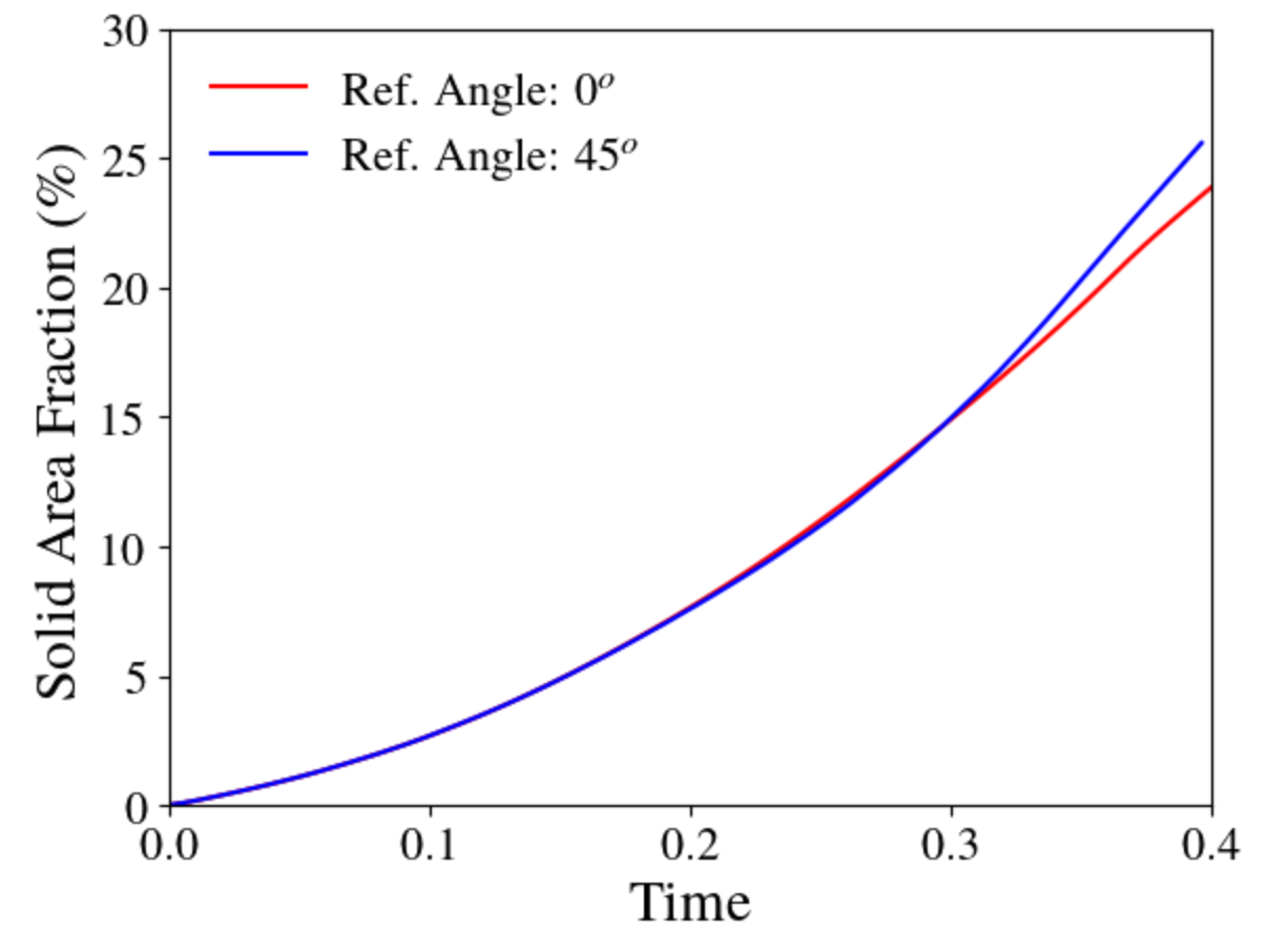
Figure 15:Dendritic growth rate.
Thus, it is important to evaluate the effect of orientation on the results by misaligning the grids. Furthermore, these effects are influenced by the discretization of the mesh. Hence, it is important to ensure that the mesh is refined enough to properly resolve the interfaces (if necessary, run a mesh convergence study). For more information about strategies to simulate multiple dendrites with varying orientation, please refer to examples by Biswas et al. Biswas et al. (2022), Warren et al. Warren et al. (2003), Dorr et al. Dorr et al. (2010), Ofori-Opoku et al. Ofori-Opoku & Provatas (2010), and Pusztai et al. Pusztai et al. (2008), among others.
Kinetics and how long to run
The amount of time the simulation should be run depends on the science or engineering question to be answered, and on the system being studied. For many classic phase field problems such as grain growth and coarsening, a characteristic feature size of the system increases with time, and the progress of microstructural evolution slows as the characteristic feature size increases. For example, in grain growth, at long times the mean grain diameter increases with time as . Another example is coarsening of spherical particles in a matrix; for sufficiently low volume fraction of particles in a matrix where solute is transported by diffusion, the mean particle radius increases with time as .
It is also useful to be aware that the system may reach a metastable or stable equilibrium state with respect to system energy, in which case no further microstructural evolution will occur for increasing simulation time. In the grain growth example, if the system evolves to a single grain, stable equilbrium has been reached. If the system evolves to a two-grain configuration with a flat grain boundary between the grains, it has reached a metastable equilibrium; the system could still lower its energy by removing the grain boundary, but in that configuration, there is no kinetic driving force to remove it from the metastable state. To monitor for such possibilities, it is useful for the simulation to periodically output the total free energy of the system; a stable or metastable equilibrium state is indicated by a constant free energy with respect to time.
References
- Biswas, S., Liu, D., Aagesen, L. K., & Jiang, W. (2022). Solidification and grain formation in alloys: a 2D application of the grand-potential-based phase-field approach. Modelling and Simulation in Materials Science and Engineering, 30(2), 025013. 10.1088/1361-651X/ac46dc
- Warren, J. A., Kobayashi, R., Lobkovsky, A. E., & Craig Carter, W. (2003). Extending phase field models of solidification to polycrystalline materials. Acta Materialia, 51(20), 6035–6058. https://doi.org/10.1016/S1359-6454(03)00388-4
- Dorr, M. R., Fattebert, J.-L., Wickett, M. E., Belak, J. F., & Turchi, P. E. A. (2010). A numerical algorithm for the solution of a phase-field model of polycrystalline materials. Journal of Computational Physics, 229(3), 626–641. https://doi.org/10.1016/j.jcp.2009.09.041
- Ofori-Opoku, N., & Provatas, N. (2010). A quantitative multi-phase field model of polycrystalline alloy solidification. Acta Materialia, 58(6), 2155–2164. https://doi.org/10.1016/j.actamat.2009.12.001
- Pusztai, T., Tegze, G., Tóth, G. I., Környei, L., Bansel, G., Fan, Z., & Gránásy, L. (2008). Phase-field approach to polycrystalline solidification including heterogeneous and homogeneous nucleation. Journal of Physics: Condensed Matter, 20(40), 404205. 10.1088/0953-8984/20/40/404205